Bourbon Secondary
Overview
There exists a number of outside forces over the recent years that have caused whiskey’s rise in popularity. Be it from advertising, dwindling stocks, demand, the secondary market, or pure magic, something has pushed prices higher and higher. Dwindling stocks are not public information, and the information that does exist isn’t quantifiable. But we can still get a decent look at the direction bourbon is heading based on the public signals available to us. In this post, I analyze the secondary market and the influence that time has had on bourbon’s price. In order to get the ball rolling, I took a page out of one of my favorite analytic blog posts of all time Why Can’t Canada Win The Stanley Cup and made heavy use out of the Google trends API to study the effect of demand on bourbon. Advertising spend was also fairly easy to collect as many spirits conglomerates are public companies that have to report their spend in various financial categories; I used Diageo’s advertising spend as a proxy for what I believe other conglomerates are spending. Lastly, in order to study the secondary market, I scraped data from a few online auction houses and piled it all together into a tidy dataset. I collected the data from all whiskey varieties (American varieties, Scotch, Japanese, and World) and then used the bourbon/rye subset of that data to make this post. The bourbon/rye data consists of final bids on unique bourbons and ryes spreading across 12 years worth of history (2005-2017). The highest bourbon bid in the dataset was ~$8,779 for a 24-year-old Bitter Truth Rye whiskey and the lowest was for US export Sheffer Fort Bourbon at a whopping ~6 dollars.
Advertising
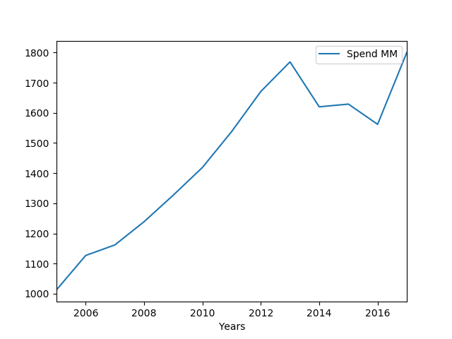
First things first, it’s important to note that the big spirit companies
have spent a lot on marketing over the past 10 years in an attempt to
take market share from the beer categories (their number one market
competitor, obviously). Note, this includes everything - all
advertisements in their portfolio - from the vodka commercial to the
paid ‘whiskey review’. Here’s Diageo, for example. They’re spending a
ton. And frankly, as you’ll see in the rest of the post, it’s working:
Demand
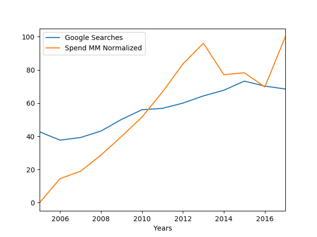
Thanks to the Google Trends API we’re able to see the direct impact of spirits marketing since 2004. We can quantify the interest in bourbon measured by the relative number of Google searches over from 2004 until present. What this plot shows is that search interest is steadily increasing as more and more people are getting familiar with bourbon. (However, you already knew that. You could feel a disruption in the bourbon force).
What’s interesting is Diageo’s spend vs. Google’s interest.
Auctions
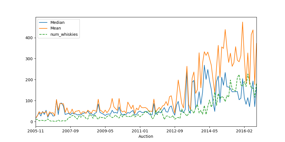 This plot represents the USD Mean bid, the USD Median bid, and
normalized number of whiskies in the given auction over time. It’s
obvious that more recently, the mean and median have become farther and
farther apart - representing “higher valued bourbons” pulling the mean
up and away from the median.
This plot represents the USD Mean bid, the USD Median bid, and
normalized number of whiskies in the given auction over time. It’s
obvious that more recently, the mean and median have become farther and
farther apart - representing “higher valued bourbons” pulling the mean
up and away from the median.
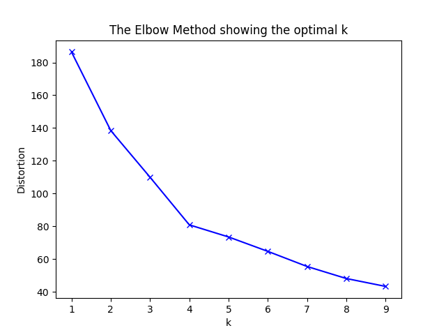
I wanted to do just a super basic clustering of prices given the brand
of bourbons to see what impact they have on pulling price away from the
median. Using the elbow method, we choose 4 clusters and then see what
brands cluster together.
from sklearn.cluster import KMeans
from sklearn import metrics
from scipy.spatial.distance import cdist
import numpy as np
import matplotlib.pyplot as plt
from sklearn.cluster import KMeans


# create new plot and data
X = df_age['usd'].values.reshape(-1, 1)

# k means determine k
distortions = []
K = range(1,10)
for k in K:
    km = KMeans(n_clusters=k).fit(X)
    distortions.append(sum(np.min(cdist(X, km.cluster_centers_, 'euclidean'), axis=1)) / X.shape[0])

# Plot the elbow
plt.plot(K, distortions, 'bx-')
plt.xlabel('k')
plt.ylabel('Distortion')
plt.title('The Elbow Method showing the optimal k')
plt.show()

# use 4 clusters
km = KMeans(4).fit(X)
pred = km.predict(X)
bourbon['clus'] = pred
smallest_grouping = np.argsort(
          [bourbon[bourbon['clus'] == i].distillery_cleaned.unique().shape[0] for i in range(0,4)]
          )[0]
print(bourbon[bourbon['clus'] == smallest_grouping].distillery_cleaned.unique())


# output
['Bitter Truth' 'Willett' 'Martin Mills' 'Van Winkle' 'Twisted Spoke'
 'Pappy Van Winkle`s' 'Old Rip Van Winkle' 'Black Maple Hill'
 'Old Fitzgerald' 'Bourbon Valley']
Bitter Truth, Willett, Martin Mills, Van Winkle, Twisted Spoke, Pappy Van Winkle`s, Old Rip Van Winkle, Black Maple Hill, Old Fitzgerald, and Bourbon Valley. No real surprises there…
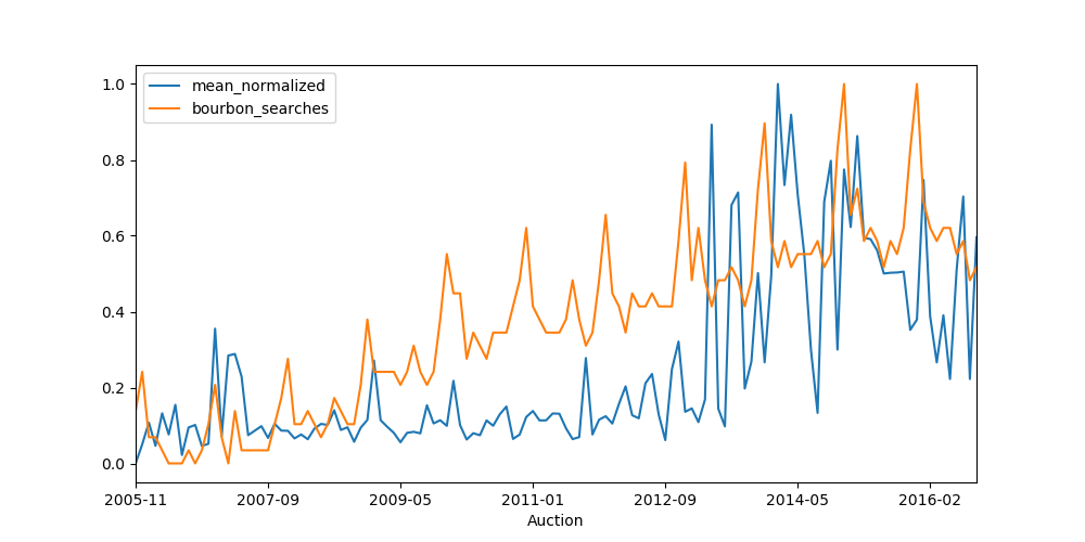
When we plot the normalized Google searches alongside the normalized mean of each auction, what’s clear is the interest in bourbon and the price of bourbon have finally converged. More people have gotten into bourbon and the cost to acquire the brown stuff has finally started to reflect the new, higher priced reality. What’s kind of cool is that given the discrepancy between the normalized mean bourbon price and Google searches during 2009-2013, one could say that with respect to interest, bourbon was mispriced during this time.
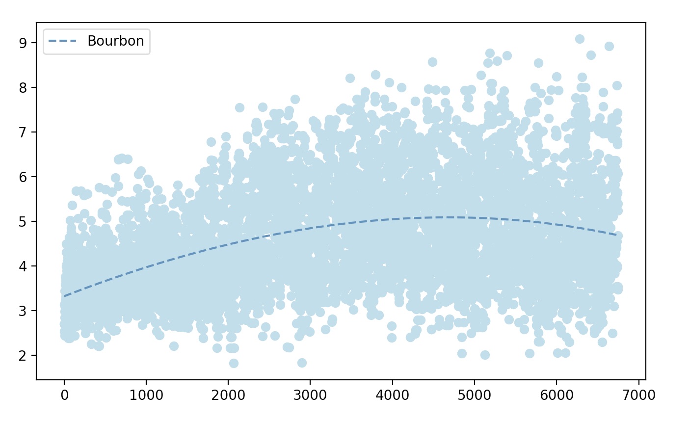
Price Plateau
Now that the basic analysis is out of the way, here are all the final purchase prices for bourbons in a nice easy log transform. Fitting a fairly naive trend-line gives us a very interesting picture. It looks like the ‘bourbon boom’ as a whole is plateauing. It’s almost as if we’ve reached equilibrium in the secondary market. There could be a million reasons for this: perhaps enough people who would happily pay thousands for a whiskey have already tried those expensive whiskies and thought: ‘you know what, once is enough’, maybe people realized good bourbon just doesn’t have to be expensive, maybe production is ramping back up and supply is finally meeting demand, again, who knows? My two cents on what I think is actually happening: people are trying to cash in on the perceived unicorn demand and are thus trying to sell just about anything. This, in turn, is flooding the secondary with mediocre or self-inflated bourbons/ryes that just aren’t considered ‘worth as much’, while the higher valued bourbons/ryes (older willetts, etc.) are starting to reach the upper bounds of what people are willing to pay for them. The influx of ‘lower-quality’ bourbons is bringing down the overall price of even ‘mediocre to good’ whiskies simply by the availability of the other options. Personally, I think this is a good thing. Flippers are not making the money they once were and are actually undermining their own scarcity-reliant cause. In essence, their strategy is leaning towards quantity and not quality to make money.
Extra Plots
For the sake of showing some interesting plots all done similarly to the previous section - log transformed over time.
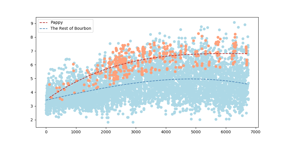
This is Pappy (only the Pappy Van Winkle lineup (15, 20, 23)) vs. the rest of bourbon/rye over time. It looks like it’s plateauing and staying steady.
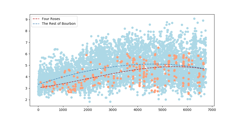
This is all Four Roses bourbons (older 70s Yellow Label all the way to new LEs and everything in between) vs. the rest of bourbon/rye over time. As one of my favorite distilleries, I’m not mad at this.
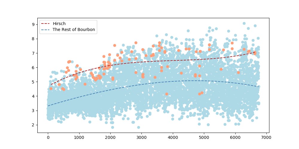
Hirsch bourbons vs. the rest of bourbon/rye over time. Seeing as the older and harder to get stuff just isn’t being reproduced, not shocked in the least at it’s trajectory.
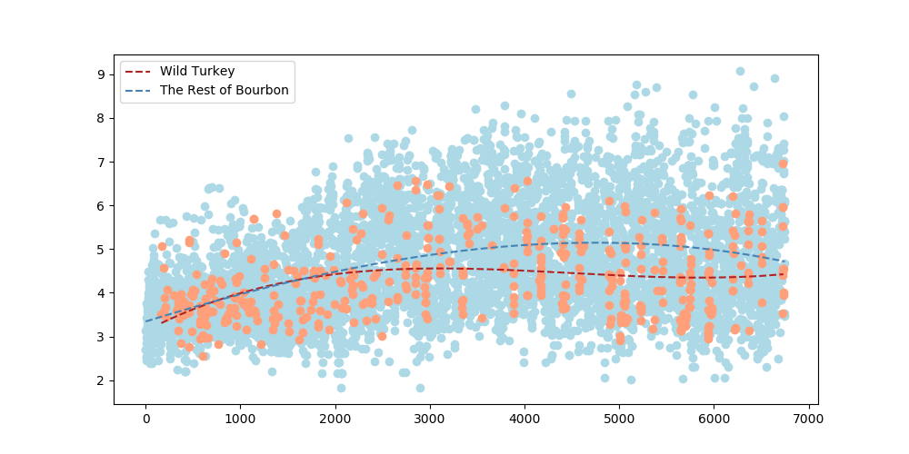
Here is Wild Turkey Bourbons and Ryes vs. the rest of bourbon/rye over time. Considering how much I love Wild Turkey, it’s nice that even the upper bound of what people are willing to pay for it isn’t anywhere close to what people are shelling out for high-valued bourbons.
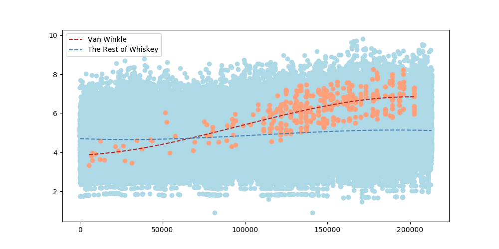
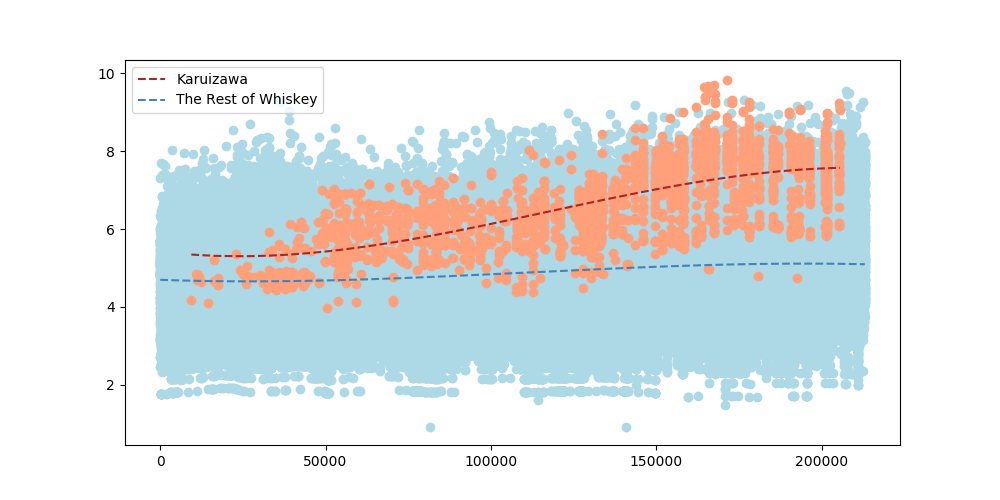
What I thought might be interesting to take all of whiskey and compare the highly-valued Van Winkle line up to some other big players in the whiskey game, Karuizawa in particular. What’s obvious is that despite it’s hegemony over bourbon, it doesn’t come close in terms of what people are willing to pay for Karuizawa. I mean who cares though, one of those distilleries was on an active volcano and stopped producing hooch in like the 80s and the other is still shelling out juice. In the end it doesn’t matter, I just like plotting stuff.
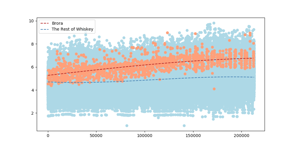
Here’s a hot take: Pappy and Brora are priced similarly in auction
markets - which, after having both - is pretty ridiculous (Both ‘good’
Brora and ‘bad’ Brora tastes better to me than any Pappy for what it’s
worth). So here it is: Buy Brora (but save some for me). It’s priced
well for relative to other hype-trains.
Driving Forces on All Whiskies
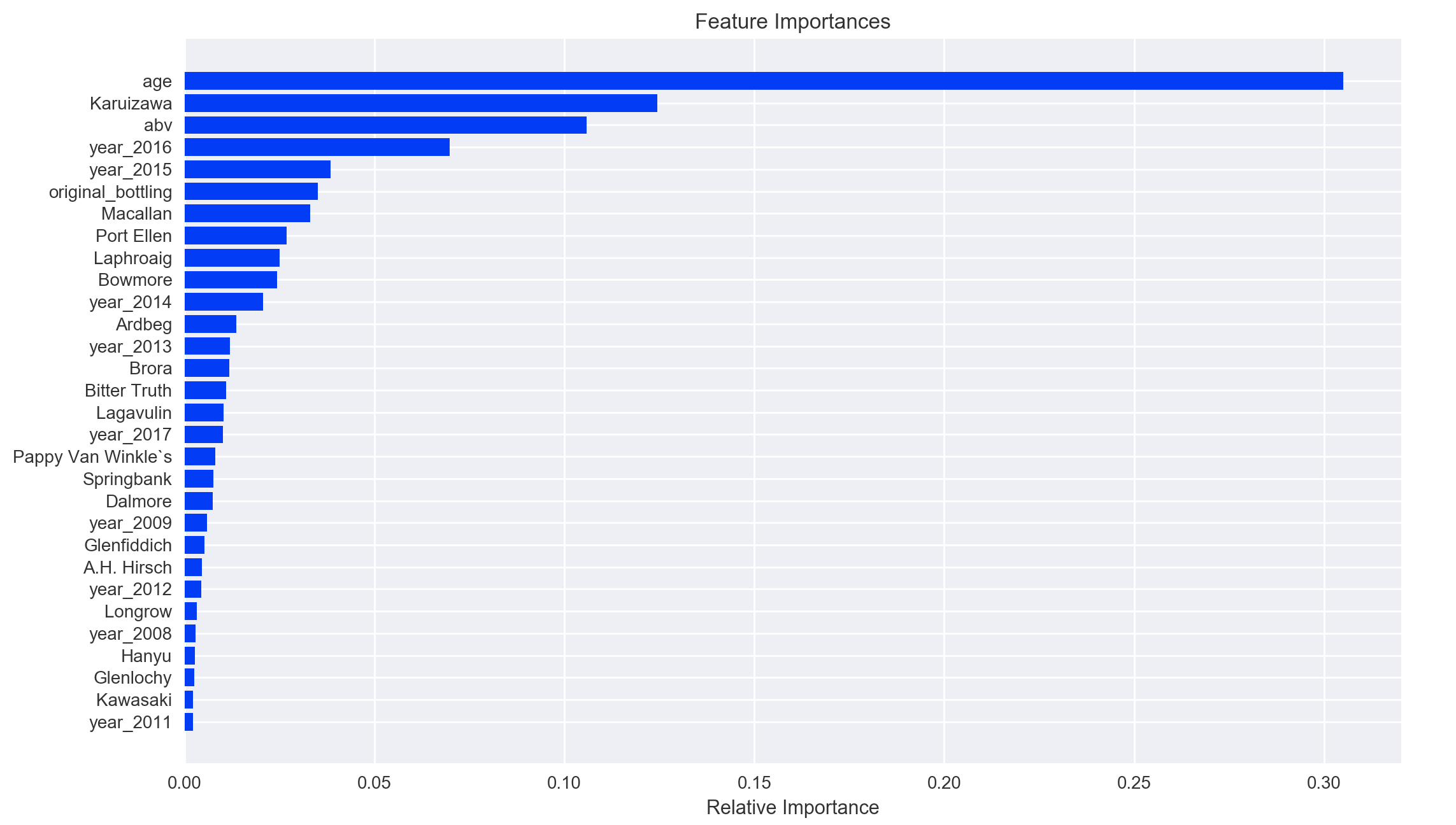
In order to see what the driving force of price is for the secondary market, I modeled the effect of the whiskey’s age, the proof, whether it was an original bottling or not (Cadenhead bottling Heaven Hill, for example), year of auction, and the distiller on the final sale price (I tried to model cask type as well, but there just wasn’t enough clean information). There are about a billion methods to do what I’m going to do, however, I chose a RandomForest because trees are inherently easier to understand for non-data whiskey lovers than more mathematically complex models (http://www.r2d3.us/visual-intro-to-machine-learning-part-1/ link for non-data people). Using a basic RandomForest model, one can easily interpret the importance each variable has on predicting the final sale price. (NOTE: this does not take into account bidding wars, bidding strategies, or number of bids per whiskey - I’ll save that for another time)
  # define our RandomForest
rf = RandomForestRegressor()

# distill (pun intended) our features from the whiskey data and make
# brand and auction year categorical
features = pd.get_dummies(data)

# fit our random forest to the dataset
rf.fit(features.values[:,1:], features.values[:,0])

# grab the feature importances from the rf
importances = rf.feature_importances_

# sort which ones are the most important [0 -> most important]
indices = np.argsort(importances)

# take the top 30 most important and make most important at 0 index
indices = indices[-30:]

# remove pandas string concatenations from data for plotting
features_names = [x.replace('distillery_cleaned_','') for x in features.columns[1:].values]

# plot title
plt.title('Feature Importances')

# plot horizontal bar
plt.barh(range(len(indices)), importances[indices], color='b', align='center')

# plot the importances
plt.yticks(range(len(indices)), np.array(features_names)[indices])

# label x axis
plt.xlabel('Relative Importance')

# plot it
plt.show()
Cool, so what does the plot below mean? First, age is the most important variable (duh). And in no particular order are the rest. Alcohol by volume: people will pay more for cask strength and higher proof whiskies. Original bottlings matter: people will pay more for an original bottling compared to that of the same spirit bottled independently (Cadenhead, Signatory, Willett, etc.). Which presents one heck of an opportunity to buy the same distillate at a discounted rate. Next is the year at which the whiskey is sold - I find this interesting; it’s basic price bubble capitalization from a supply/demand perspective, and lastly, at no surprise to anyone, is brand power. All of this is pretty much confirming what we already believed: in the context of marketing and demand, 2014 onwards have benefited from increased interest in whiskey where the demand for certain brands has a direct relationship with price. People are wanting higher proof distillate from specific brands and will pay more if it is bottled by the particular distillery.
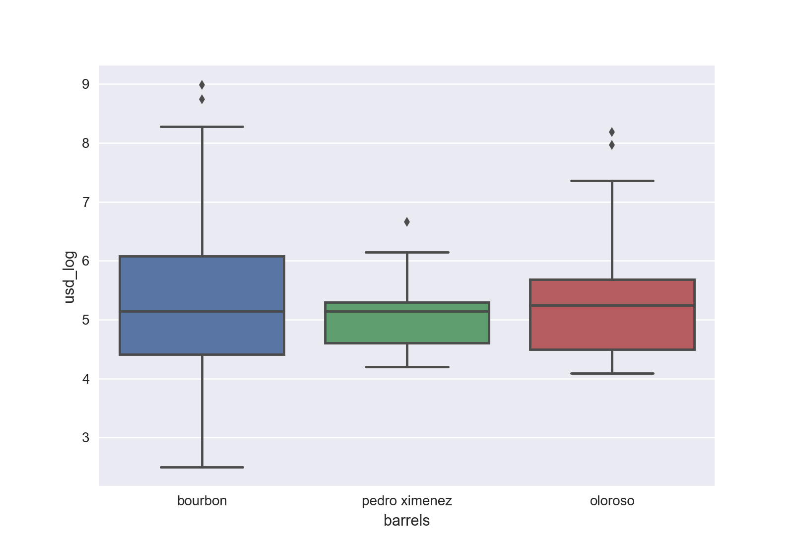
 Somewhat related, I tried to use barrel-type as a variable, but there
just wasn’t enough clean information to incorporate into the
over-arching model. However, what information that did exist basically
says that scotches aged in Pedro Ximenez barrels are more evenly
distributed with respect to price than bourbon or oloroso barrels.
Considering my love for all things Pedro Ximenez, I found this pretty
interesting.
Somewhat related, I tried to use barrel-type as a variable, but there
just wasn’t enough clean information to incorporate into the
over-arching model. However, what information that did exist basically
says that scotches aged in Pedro Ximenez barrels are more evenly
distributed with respect to price than bourbon or oloroso barrels.
Considering my love for all things Pedro Ximenez, I found this pretty
interesting.
 So in the end, what does this all mean? Well, basically, Age + ABV + OB
- Brand + Timing = Price. Go figure. The alternate take is that outside the top brands, there exist many lower cost (and better tasting) options for cask-strength, high aged, originally bottled spirit. Now most people have never tried the wealth of distilleries in existence, and that includes the big players - the Karuizawa’s, 80s Macallans, or Stitzel-Wellers, so maybe next time, rather than wasting your time hunting down a bottle of this stuff (or any in-demand juice), try 20 different whiskies for the same price. I personally think that it can be a lot less of a risk than it may seem to buy a lesser known brand than to spend $1500 (or even whatever it goes for at MSRP) on 23 year old Pappy Van OakJuice. All in all, when you have increased demand, whiskey hoarders, ‘dwindling supply’, advertising - sometimes in the form of bought and paid for ‘reviewers’ all working at the behest of large brands, it’s easy to get caught up in thinking that these bottles of liquid are worth the money others are paying for them. However, you’re a smart person, you’re informed, you’re not going to get caught up in the brand hype. In fact, you’re going to set out and do more blind taste tests to truly see if all this crap is just hype or actually worth it to your wallet.