The Model Knows When It’s Moving. That Doesn’t Mean You Can Tell It to Stop.
==================
What two mechanistic-interpretability studies taught us about controlling idle motion in streaming Wan video models.
on the flight back from a week in sf, after trying to get a demo together that just would not cooperate, i did some retrospective reading to understand exactly how the pieces fit together. time to reverse a claude-induced critical-thinking lobotomy.
why did this seemingly benign model always produce motion? 99.9% of life is stillness, yet every video model produces idle movement: camera movement, subject movement, world movement, there is always movement. there’s never just stillness. even from the perspective of a system like Rolling-Sink, we should see continuous stillness based on reality, no? i get that it enforces motion, but that’s not reality.
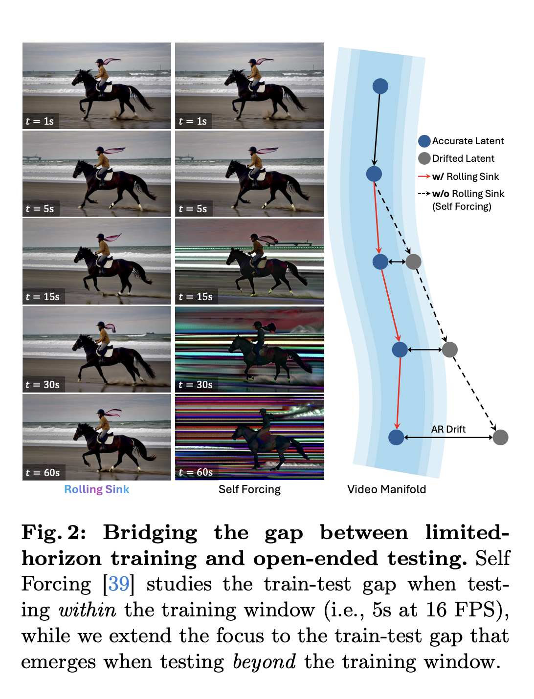
so the problem was trying to get an avatar model to stay put. the solution is still TBD, tbh; perhaps it needs training from scratch. but could we enforce reality norms post hoc? could we get things to “be still” when appropriate without post-training? who knows, but that question led me to look at the problem in a different light:
why is this avatar twitching, and what can i do to fix it?
let’s look at the desired behavior of an avatar that’s being streamed: it should gesture while speaking, shift naturally, react, and move when the performance calls for it. this implicitly means it should know when not to move.
during early streaming LiveAvatar experiments, we kept seeing a specific failure mode: shifting, gesturing, or moving spasmodically while idle.
it made me think: does the video model internally know how much motion it is producing—and, if it does, can we use that representation to control the result?
with Claude’s help, i ran two studies to find out
the first examined the Wan 14B speech-to-video model. the second repeated and expanded the experiment on a much smaller Wan2.1 T2V 1.3B model. both systems used Rolling-Sink to support continuous, long-horizon generation.
what we learned:
motion is almost perfectly readable from the models’ hidden states. but a readable representation is not automatically a clean control knob.
why streaming video drifts (generally)
duh. video models are nearly exclusively trained on movement data: cameras, subjects, etc. that’s very useful when we want dynamic performance, but it can be bad when we’re looking for subtle stillness.
this is compounded in streaming: a normal video model generates a bounded clip. a streaming system must continue beyond that horizon while maintaining identity, composition, and temporal context.
in the context of something like rolling-sink, context is through a persistent attention KV cache. in the implementation we studied, it combined three mechanisms:
- a cache that writes new keys and values while evicting old ones;
- a rolling window that re-injects selected earlier states; and
- a global positional offset that keeps increasing across generated clips.
these mechanisms help the model continue indefinitely, but they can also alter the model’s motion behavior over time. so our first goal became not wanting to remove movement from the model entirely, it was to separate intentional motion from unwanted accumulated motion.
reading motion from the model
ok claude, here are the parameters of <the thing> i want to understand, can you help?
Claude, take it away
We began with a straightforward probe.
For a set of still and movement-heavy prompts, we collected activations from each transformer layer. We spatially pooled them into per-frame features; one run used their temporal differences while the other averaged them over time. We then trained a linear ridge-regression probe to predict the generated clip’s motion score.
If motion were only an emergent property of the final pixels, with no stable internal representation, this probe should have performed poorly. It did not.
In the 14B model, every transformer layer was highly predictive. Probe R² rose from 0.943 at the first layer to 0.9965 at layer 39, the final block. The final five layers all exceeded R²=0.995.
The smaller model told the same story. In the 1.3B model, R² rose from 0.875 at layer 0 to 0.9925 at layer 28 of 30. Still, generic, and movement prompts also separated clearly in both latent velocity and decoded optical flow.
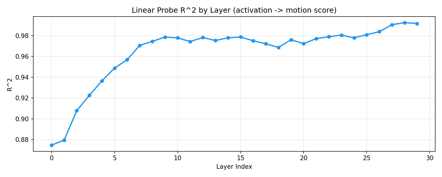
This is a remarkably robust result across a large difference in model size and conditioning. Motion is not an opaque side effect that appears only at decode time. The DiT develops a progressively refined internal representation of how much movement its output will contain.
Knowing is not the same as controlling
The obvious next move was activation steering.
We took the direction learned by the linear probe and added or subtracted it from the model’s residual stream. If the probe had found a clean, signed “motion axis,” moving in one direction should increase motion and moving in the other should reduce it.
That is not what happened.
In the 14B model, activation patching at the final layer changed the motion score, evidence that the representation participates in the computation. But subtracting the fitted direction increased motion at every tested strength. Adding the direction slightly improved pixel MSE in a later test while making optical flow roughly 38% worse.
The 1.3B model was more steerable, but only in a narrow range. Alpha values of 0.5 and 1.0 reduced its latent motion proxy by approximately 45-47%. At alpha 2.0, the benefit almost disappeared. At alpha 5.0, motion increased by more than 61%. Some negative alpha values also reduced motion.
That sign ambiguity matters. It suggests that the probe found a motion-associated direction of variance, or one projection through a broader motion subspace, rather than a single scalar feature labeled “more motion.”
The broader lesson is important beyond video:
Linear decodability, causal participation, and monotonic controllability are three different claims.
A feature can be easy to predict, and even causally involved, without providing a safe intervention direction.
The upstream causes were more useful
The most actionable results came from studying what fed the motion representation in the first place.
For the LiveAvatar experiment, we generated 20 sequential clips under four conditions. Every condition used the same LiveAvatar 14B model and LoRA; we varied whether Rolling-Sink was enabled and whether the audio input contained low-amplitude “breathing” noise or true silence.
| LiveAvatar 14B condition | Pixel MSE | Optical flow | Pixel MSE relative to NoRS + silence |
|---|---|---|---|
| Rolling-Sink enabled + breathing audio | 882.6 | 1.761 | 7.67x |
| Rolling-Sink enabled + silence | 318.1 | 0.828 | 2.76x |
| Rolling-Sink disabled + breathing audio | 243.7 | 1.329 | 2.12x |
| Rolling-Sink disabled + silence | 115.1 | 0.726 | 1.00x |
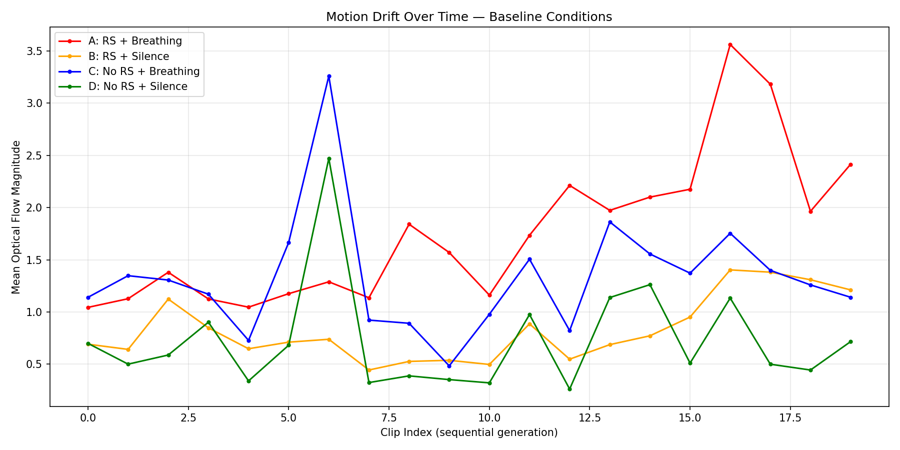
Two independent effects were visible.
First, the audio-conditioned model treated even quiet breathing noise as a real signal. Those nonzero audio embeddings produced roughly twice as much motion as silence. This is reasonable from the model’s perspective: audio is supposed to drive a speech-to-video actor. “Almost silent” and “zero conditioning” are not the same input.
Second, Rolling-Sink introduced cumulative drift. Without it, motion fluctuated but remained broadly stationary. With it, movement tended to grow across successive clips. The global positional offset was a particularly strong suspect: it increased monotonically even as generation moved far beyond the horizon seen during training.
Together, Rolling-Sink and breathing audio produced 7.67 times the pixel MSE of the clean LiveAvatar NoRS-and-silence baseline. The factors did not merely add; they interacted.
What actually worked
The most reliable intervention was EMA latent anchoring.
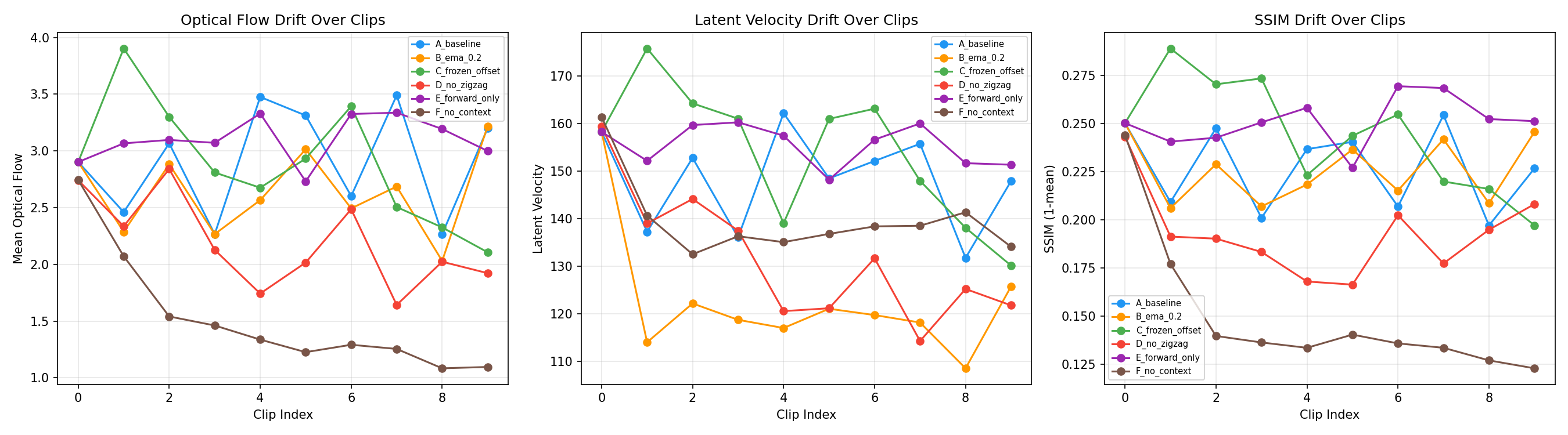
After each generated clip, we re-encoded the last frame and blended that drifted reference toward an original rest-pose anchor. With an alpha of 0.2, the 14B experiment reduced pixel MSE by 69% and optical flow by approximately 48%.
Unlike direct denoising manipulation, anchoring did not try to suppress every frame-to-frame change. It established a slow restorative force: the actor could still move locally, but long-horizon generation was discouraged from wandering arbitrarily far from its resting manifold.
The smaller model replicated the result, though less dramatically. EMA reduced its latent motion proxy by 17.5% and decoded optical flow by about 9% while remaining visually stable.
Freezing the Rolling-Sink global offset was also effective in the 14B study, reducing motion by approximately 56% against a matched ten-clip baseline. The same intervention did not reproduce strongly in the 1.3B implementation, which may reflect differences in modality, sequence length, or the exact Rolling-Sink code path.
The 1.3B model surfaced another useful result: disabling zigzag behavior reduced the latent proxy by 11.3% and optical flow by approximately 25%. This supports the hypothesis that alternating re-injection direction can create periodic recasting or instability.
What the intervention code actually touched
The experiments did not require retraining either model. They instrumented a small number of inference-time seams in the streaming pipeline:
| Question | Code path | Intervention |
|---|---|---|
| Where is motion represented? | DiT transformer-block outputs | Forward hooks collected spatially pooled activations. |
| Can the representation steer generation? | A selected block’s residual output | The fitted ridge direction was added or subtracted from every token. |
| Can long-horizon drift be restored? | Reference latents passed between clips | The last frame was VAE-encoded and blended toward a rest-pose anchor. |
| Do positions accumulate motion? | Rolling-Sink KV-cache position counters | Global/local offsets were frozen, reset, or periodically wrapped. |
| Does re-injection add instability? | The context-update call and self-attention re-injection branch | Zigzag was bypassed or constrained to forward-only traversal. |
| Does “idle” audio still drive motion? | Speech-to-video audio conditioning | The same sequence was run with a low-noise waveform and an all-zero waveform. |
The full 1.3B runner is included in
app_motion_probe_1_3b.py.
The 14B runner was coupled to a separate LiveAvatar implementation, so the
snippets below show that integration in implementation-neutral form rather than
reproducing the surrounding model source.
Collecting activations and fitting the probe
The collector attached a PyTorch forward hook to each DiT block. A block emits
[batch, sequence, hidden]; because the number of spatial tokens per frame was
known, we could recover the frame dimension and average over space:
activations = {}

def capture(layer, tokens_per_frame):
    def hook(_module, _inputs, output):
        batch, sequence, hidden = output.shape
        frames = sequence // tokens_per_frame
        per_frame = output.detach().view(
            batch, frames, tokens_per_frame, hidden
        ).mean(dim=2)
        activations[layer] = per_frame  # [B, T, C]
    return hook

handles = [
    block.register_forward_hook(capture(i, tokens_per_frame=1560))
    for i, block in enumerate(pipeline.generator.model.blocks)
]
For the 1.3B run, the per-frame states were averaged over time and a ridge model predicted the clip’s latent-velocity target. The fitted coefficients became the candidate steering direction:
from sklearn.linear_model import Ridge

features = activations[layer].float().cpu().numpy().mean(axis=1)
probe = Ridge(alpha=1.0).fit(features, motion_targets)
motion_direction = probe.coef_
This was deliberately a simple probe. Its purpose was to test whether motion was linearly readable, not to claim that one vector fully describes the model’s motion circuit.
Steering the residual stream
Steering used another forward hook at the best-performing layer. The same vector was broadcast across every spatiotemporal token:
direction = torch.as_tensor(
    motion_direction,
    dtype=torch.bfloat16,
    device=device,
)

def steer(_module, _inputs, output, alpha=1.0):
    return output - alpha * direction[None, None, :]

handle = pipeline.generator.model.blocks[layer].register_forward_hook(steer)
try:
    video = generate(prompt)
finally:
    handle.remove()
Sweeping alpha in both directions produced the non-monotonic results described
above. The hook is small; choosing a safe direction and magnitude is the hard
part.
EMA anchoring between clips
The 14B intervention acted on the reference latent supplied to the next clip. After generation, it encoded the last frame, then pulled that drifted reference strongly toward the original rest pose:
rest_anchor = encode_reference(original_image)
reference_for_next_clip = rest_anchor

for clip_index in range(num_clips):
    frames = generate_clip(
        preserve_kv_cache=clip_index > 0,
        ref_latents_override=reference_for_next_clip,
    )

    drifted_reference = vae.encode(to_vae_tensor(frames[-1]))
    reference_for_next_clip = (
        0.8 * rest_anchor + 0.2 * drifted_reference
    )
The smaller-model experiment anchored generated blocks rather than the next clip’s reference input:
denoised = 0.8 * denoised + 0.2 * first_clip_anchor
Both experiments called the setting “alpha 0.2,” but alpha multiplied opposite operands. In the 14B run it retained 20% of the drifted reference; in the 1.3B run it injected 20% of the anchor. The equation—not the parameter name—is the portable specification.
Bounding Rolling-Sink position state
Rolling-Sink state lived in slightly different places in the two implementations. The 1.3B pipeline exposed position tensors in each block’s KV cache, so the ablation reset them at clip boundaries:
def reset_rs_positions(pipeline):
    for cache in pipeline.kv_cache1:
        cache["global_end_index"].zero_()
        cache["local_end_index"].zero_()

sequence_start = 0
for clip_index in range(num_clips):
    if clip_index and clip_index % reset_every == 0:
        reset_rs_positions(pipeline)
        sequence_start = 0
    generate_next_clip(
        preserve_kv_cache=clip_index > 0,
        current_start=sequence_start,
    )
    sequence_start += frames_per_clip
The 14B path kept a model-level _rs_global_token_offset. The corresponding
intervention set or wrapped that counter on every block that exposed it. The
standalone helpers are in
interventions.py.
Resetting position metadata while retaining cached keys and values is an ablation, not automatically a production-safe operation. A production policy needs to preserve whatever invariants its positional encoding expects.
Bypassing zigzag re-injection
In the public 1.3B runner, a zero-timestep context-update pass triggers the Rolling-Sink re-injection path. The no-zigzag condition used a nonzero sentinel for that update while leaving normal denoising unchanged:
context_timestep = -1 if skip_zigzag else config.context_noise  # normally 0

pipeline.generator(
    noisy_image_or_video=denoised,
    timestep=torch.full((1, frames_per_block), context_timestep, device=device),
    kv_cache=pipeline.kv_cache1,
    crossattn_cache=pipeline.crossattn_cache,
    current_start=current_start,
    conditional_dict=conditioning,
)
The forward-only condition additionally required the self-attention re-injection branch to honor a direction override. That integration point is why monkey-patching the wrong symbol in the earlier 14B ablation produced byte-identical outputs: the actual call site still held its original function binding.
Testing whether idle audio was really idle
The audio ablation changed only the waveform passed into the speech-to-video conditioner. One input was exactly zero; the other was low-amplitude white noise with a slow envelope:
samples = int(seconds * sample_rate)
t = np.arange(samples, dtype=np.float32) / sample_rate

silence = np.zeros(samples, dtype=np.float32)

rng = np.random.default_rng(seed)
envelope = 1.0 + 0.3 * (0.5 * np.sin(2 * np.pi * 0.15 * t))
breathing = (
    0.005 * rng.standard_normal(samples) * envelope
).astype(np.float32)
Those arrays were saved as WAV files and passed through the same audio encoder. The point was not that this particular synthetic breathing signal was special; it was that a waveform that sounded negligible to us was not negligible to the conditioning network.
The damping control that failed
Finally, velocity damping modified the denoising trajectory itself:
previous_noisy = noisy_input.clone()
_, denoised = pipeline.generator(
    noisy_image_or_video=noisy_input,
    conditional_dict=conditioning,
    timestep=timestep,
    kv_cache=pipeline.kv_cache1,
    crossattn_cache=pipeline.crossattn_cache,
    current_start=current_start,
)
denoised = previous_noisy + beta * (denoised - previous_noisy)
This compact intervention is the one that produced flicker. It constrained the step update, but did not distinguish coherent motion from destructive high-frequency error.
A failed intervention worth remembering
Latent-velocity damping looked good before it looked terrible.
In an early, short 14B probe, beta=0.1 reduced the latent motion metric by 15.9%. If we had stopped at that metric, we might have declared it the winner.
Once we decoded multi-clip sequences, the failure was obvious. Damping disrupted the denoising trajectory and created continuous flicker. Pixel MSE increased by 62% at beta=0.1 and 51% at beta=0.3.
The 1.3B study confirmed the failure: every tested damping value increased motion. Combining damping with otherwise useful steering and EMA controls left only a 1.82% improvement because damping canceled the benefits.
This is why video interventions need multiple measurements. Latent velocity is cheap and, in our 1.3B results, correlated strongly with optical flow and SSIM. But a model can reduce one proxy by replacing coherent motion with high-frequency jitter. The metric improves while the video gets worse.
What this means for controllable virtual actors
The practical goal is not a motionless avatar. It is an actor whose movement is appropriate to context.
Our current production-oriented recommendations are:
- Use true silence during genuine idle rather than low-amplitude synthetic breathing audio.
- Add a tunable rest-pose anchor, with EMA alpha around 0.2 as a starting point.
- Cap or periodically reset the Rolling-Sink global positional offset.
- Test forward-only or disabled re-injection using method-level patches that definitely reach the attention call site.
- Use latent velocity as a cheap online detector, but validate every control against decoded optical flow, flicker, identity retention, and human judgment.
- Avoid latent-velocity damping as currently formulated.
- Treat activation steering as an experimental expressive lever with bounded strength, not a universally safe “motion slider.”
There may eventually be many useful steering directions: motion intensity, camera behavior, gaze, expression, pose, or interaction dynamics. The small model’s strong probe performance makes that research direction especially interesting. But each direction needs causal and visual validation—not merely a high probe score.
Important limitations
These were exploratory engineering studies, not controlled training runs.
The two models used different modalities, architectures, sequence shapes, and motion scales, so their raw numbers should not be compared directly. The 14B experiment used LiveAvatar’s TPP-capable graph pipeline, but deliberately ran it on one H100 with world size one, sequence parallelism disabled, one DiT GPU, and all denoising timesteps executed on the same rank. It therefore does not prove that the exact drift ratios carry over to LiveAvatar’s multi-GPU timestep-parallel production topology.
One early 14B run also exposed a state-reset bug, and two re-injection ablations were invalid because a monkey patch did not reach an import-time function binding. We excluded those invalid comparisons from our conclusions.
The next rigorous experiment should repeat the corrected ablations across multiple seeds and both single-GPU and production TPP topologies. It should factor audio, positional-offset policy, re-injection mode, anchoring strength, and steering strength while measuring motion, identity, quality, and human preference.
The broader lesson
The most exciting result is not simply that we reduced idle motion. It is that motion appears to be an exceptionally legible internal variable in video DiTs, even at 1.3B parameters.
The most useful result is the warning attached to it.
The model knows when it is moving. But reading that knowledge and controlling the process are different problems. The best interventions came from understanding the upstream system—conditioning, cache geometry, positions, and long-horizon state—not from pushing harder on the first direction a probe gave us.
That distinction is likely to matter as video models become more interactive. Controllable virtual actors will need more than the ability to generate motion. They will need the ability to choose the right motion, at the right time, for the right reason.